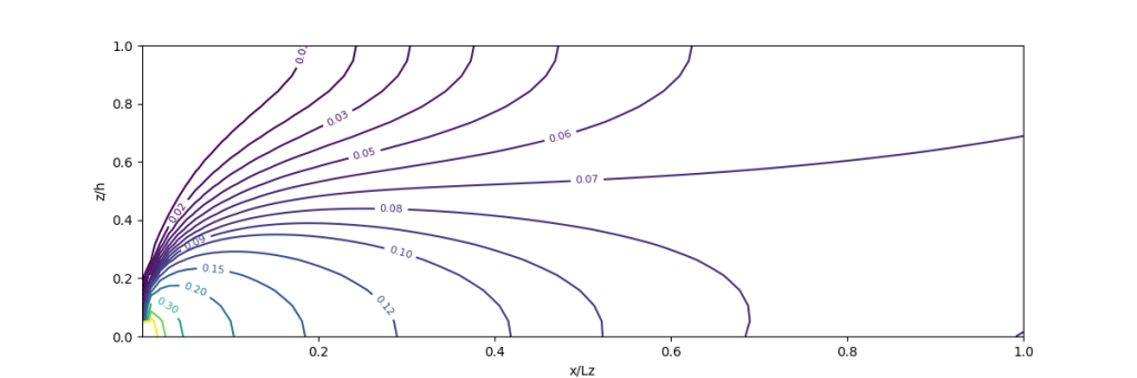
Source code di bawah ini memplotkan kontur konsentrasi polutan yang diperoleh dari penyelesaian analitik persamaan transpor konveksi-difusi di sungai. Lihat bahan ajar mata kuliah Dinamika Aliran dan Transfer Massa. Program dituliskan dalam bahasa pemrograman Python. Program dibuat sederhana agar mudah dibaca dan dimodifikasi oleh pengguna.
Konveksi-Difusi Vertikal (di Near-field Zone)
Exercise 8B
import numpy as np
import matplotlib.pyplot as plt

# Dinamika Aliran dan Transfer Massa
# Konveksi-difusi vertikal
# Exercise 8B

# data
Q = 103.7
U = 1.05
B = 90.6
h = 1.09
ustar = 0.07
Sf = 0.0005
T = 10.
C = 10.
Qu = 0.5
Tu = 20.
Cu = 30.
xsi = 0.4

# hitungan
A = B * h
etz = 0.067 * h * ustar
Lz = xsi * U * h * h / etz
tz = Lz / U
nx = 100
nz = 20
# dx = Ly / nx
# dz = h / nz
print("Ly ", Lz, "m")
print("ty", tz, "s")
x = np.linspace(0.01, Lz, nx)
z = np.linspace(0.0, h, nz)
c = np.zeros((len(x), len(z)), dtype=float)
Gu = Cu * Qu
i = 0
for xc in x:
    j = -1
    for zc in z:
        j = j + 1
        c[i, j] = Gu / B / np.sqrt(4 * np.pi * etz * xc * U) * np.exp(-1. * zc * zc * U / (4. * etz * xc))
        zz = zc - 2 * h
        c[i, j] = c[i, j] + Gu / B / np.sqrt(4 * np.pi * etz * xc * U) * np.exp(-1. * zz * zz * U / (4. * etz * xc))
        zz = zc
        c[i, j] = c[i, j] + Gu / B / np.sqrt(4 * np.pi * etz * xc * U) * np.exp(-1. * zz * zz * U / (4. * etz * xc))
    i = i + 1
tulis_teks = " ".join(f"{val:7.4f}" for val in z)
print(f"          {tulis_teks}")
ii = 0
for row in c:
    tulis_teks = " ".join(f"{val:7.4f}" for val in row)
    print(f"{x[ii]:9.4f} {tulis_teks}")
    ii = ii + 1
print("Selesai hitungan konsentrasi")

# plot kontur konsentrasi
x = x / Lz
z = z / h
print("cmin, cmaks ", np.min(c), np.max(c))
zi, xi = np.meshgrid(z, x)
kontur1 = ([0.001])
kontur2 = np.linspace(0.01, 0.20, 20)  # nilai-nilai c yg akan di-kontur-kan
kontur3 = ([0.25, 0.3, 0.4, 0.5, 0.6])  # nilai-nilai c yg akan di-kontur-kan
kontur = np.hstack((kontur1, kontur2, kontur3))

plt.figure(figsize=(12, 6))
plot = plt.contour(xi, zi, c, levels=kontur, cmap='viridis')
plt.xlabel('x/Ly', fontsize=14)
plt.ylabel('z/h', fontsize=14)
plt.clabel(plot, inline=1, fontsize=8)

plt.savefig('kontur_kondif_vertikal.png')
plt.show()
Konveksi-Difusi Transversal (di Mid-field Zone)
Exercise 8C
![]()
![]()
import numpy as np
import matplotlib.pyplot as plt

# Dinamika Aliran dan Transfer Massa
# Konveksi-difusi transversal
# Exercise 8C

# data
Q = 103.7
U = 1.05
B = 90.6
h = 1.09
ustar = 0.07
Sf = 0.0005
Qu = 0.5
Cu = 30.
# Posisi source
# y0 = B / 2.
y0 = 0.
if y0 == 0.0:
    xsi = 0.5
else:
    xsi = 0.1
print("xsi", xsi)

# hitungan
A = B * h
ety = 0.6 * h * ustar
print("ety", ety)
Ly = xsi * U * B * B / ety
ty = Ly / U
Ly = np.round(Ly / 1000, 0) * 1000.
ty = np.round(ty / 3600, 0) * 3600.
print("Ly ", Ly, "m", Ly / 1000, "km")
print("ty", ty, "s", ty / 3600, "jam")
nx = 200
ny = 200
x = np.logspace(-4, 0, nx)
y = np.linspace(B, 0., ny)
c = np.zeros((len(y), len(x)), dtype=float)
Gu = Cu * Qu
j = 0
for col in x:
    #    xc = np.power(10, col) * Ly
    xc = col * Ly
    koef = Gu / h / np.sqrt(4 * np.pi * ety * xc * U)
    i = -1
    for row in y:
        i = i + 1
        yc = row - y0  # original source
        c[i, j] = koef * np.exp(-1. * yc * yc * U / (4. * ety * xc))
        yc = row - (2. * B - y0)  # image source kiri
        c[i, j] = c[i, j] + koef * np.exp(-1. * yc * yc * U / (4. * ety * xc))
        yc = row - y0  # image source kanan
        c[i, j] = c[i, j] + koef * np.exp(-1. * yc * yc * U / (4. * ety * xc))
    j = j + 1
tulis_teks = " ".join(f"{val:7.4f}" for val in x)
print(f"          {tulis_teks}")
tulis_teks = " ".join(f"{val * Ly / 1000:7.4f}" for val in x)
print(f"          {tulis_teks}")
ii = 0
for row in c:
    tulis_teks = " ".join(f"{val:7.4f}" for val in row)
    print(f"{y[ii]:9.4f} {tulis_teks}")
    ii = ii + 1
print("Selesai hitungan konsentrasi")

# plot kontur konsentrasi
y = y / B
print("cmin, cmaks ", np.min(c), np.max(c))
xi, yi = np.meshgrid(x, y)
# nilai-nilai kontur yang akan diplotkan
kontur1 = np.linspace(0.001, 0.01, 2)
kontur2 = np.linspace(0.1, 1, 10)
kontur3 = ([2.0, 3.0])
kontur = np.hstack((kontur1, kontur2, kontur3))

plt.figure(figsize=(12, 6))
plot = plt.contour(xi, yi, c, levels=kontur, cmap='viridis')
plt.xscale('log')
plt.xlabel('x/Ly', fontsize=14)
plt.ylabel('y/B', fontsize=14)
plt.clabel(plot, inline=1, fontsize=8)

plt.savefig('kontur_kondif_transversal.png')
plt.show()